Search Box

Except using the Find function in Excel, actually you can create your own search box for searching needed values easily.

Search for the desired location and enter information in the record. How to make a custom form. How to display a custom form. How to format a custom form.

This example teaches you how to create your own search box in Excel. If you are in a hurry, simply download the Excel file.

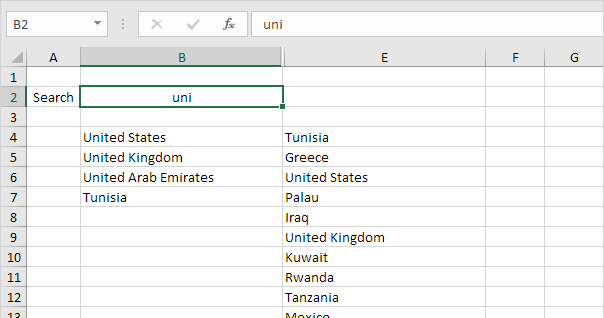
This is what the spreadsheet looks like. If you enter a search query into cell B2, Excel searches through column E and the results appear in column B.

To create this search box, execute the following steps.

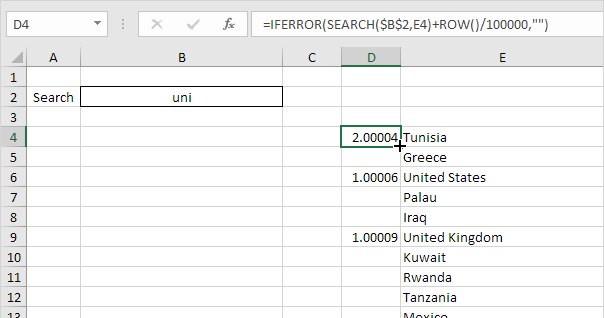
1. Select cell D4 and insert the SEARCH function shown below. Create an absolute reference to cell B2.

2. Double click the right corner of cell D4 to quickly copy the function to the other cells.

Explanation: the SEARCH function finds the position of a substring in a string. The SEARCH function is case-insensitive. For Tunisia, string “uni” is found at position 2. For United States, string “uni” is found at position 1. The lower the number, the higher it should be ranked.

3. Both United States and United Kingdom return the value 1. To return unique values, which will help us when we use the RANK function in a moment, slightly adjust the formula in cell D4 as shown below.

4. Again, double click the right corner of cell D4 to quickly copy the formula to the other cells.

Explanation: the ROW function returns the row number of a cell. If we divide the row number by a large number and add it to the result of the SEARCH function, we always have unique values. However, these small increments won't influence the search rankings. United States has a value of 1.00006 now and United Kingdom has a value of 1.00009. We also added the IFERROR function. If a cell contains an error (when a string cannot be found), an empty string ("") is displayed.

5. Select cell C4 and insert the RANK function shown below.

6. Double click the right corner of cell C4 to quickly copy the formula to the other cells.

Explanation: the RANK function returns the rank of a number in a list of numbers. If the third argument is 1, Excel ranks the smallest number first, second smallest number second, etc. Because we added the ROW function, all values in column D are unique. As a result, the ranks in column C are unique too (no ties).

7. We are almost there. We'll use the VLOOKUP function to return the countries found (lowest rank first, second lowest rank second, etc.) Select cell B4 and insert the VLOOKUP function shown below.

8. Double click the right corner of cell B4 to quickly copy the formula to the other cells.

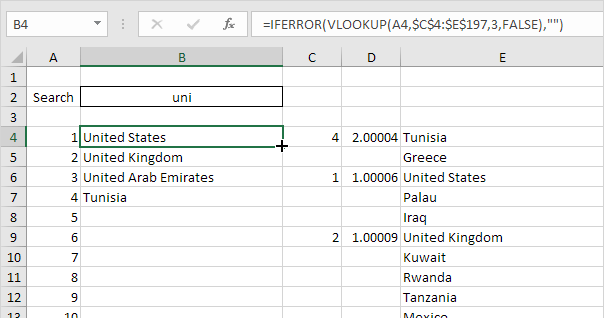
9. Change the text color of the numbers in column A to white and hide columns C and D.

Result. Your own search box in Excel.