Superscript and Subscript

Applying superscript and subscript format in Excel isn’t straightforward unlike in Microsoft Word.

It’s understandable. Microsoft Word is a text processor while Excel is a spreadsheet software, which mostly deals with data and numbers.

However, it does have a lot of tricks of its own.

It's easy to format a character as superscript (slightly above the baseline) or subscript (slightly below the baseline) in Excel.

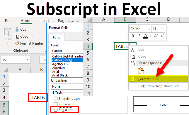
1. For example, double click cell A1.

2. Select the value 2.

3. Right click, and then click Format Cells (or press Ctrl + 1).

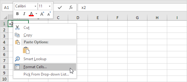
The ‘Format Cells’ dialog box appears.

4. On the Font tab, under Effects, click Superscript.

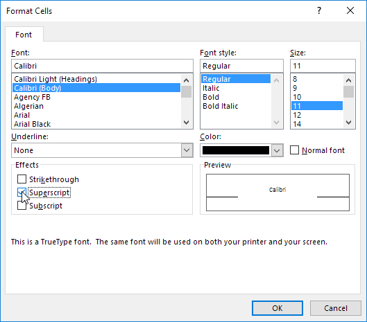
5. Click OK.

Result:

6. Needless to say, a superscript effect cannot return a result. To square a number, use a formula like this:

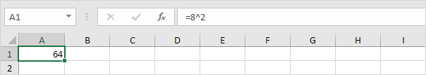
Note: to insert a caret ^ symbol, press SHIFT + 6.

7. To format a character as subscript (slightly below the baseline), repeat steps 1-5 but at step 4 click Subscript.

Result:

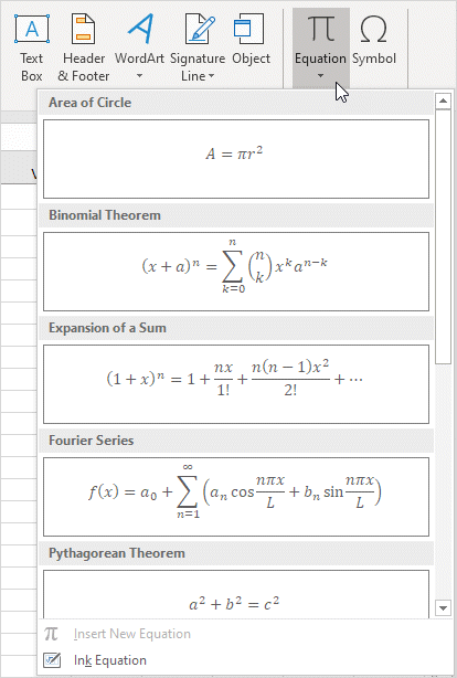
8. Did you know that you can also insert equations in Excel? On the Insert tab, in the Symbols group, click Equation.

Note: equations in Excel are floating objects and do not return results.