Check Mark ✓

You can easily insert a check mark (also known as a “tick mark”) in Excel.

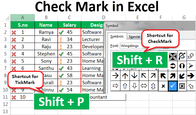
To insert a check mark symbol in Excel, simply press SHIFT + P and use the Wingdings 2 font. You can also create a check list that uses check boxes.

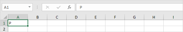
1. Select cell A1 and press SHIFT + P to insert a capital P.

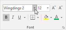
2. On the Home tab, in the Font group, select the Wingdings 2 font. To insert a fancy check mark, change the font color to green, change the font size to 12 and apply bold formatting.

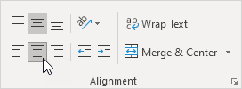
3. On the Home tab, in the Alignment group, use the Align buttons to center the check mark horizontally and vertically.

Result. A check mark in Excel.

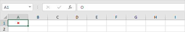
4. To insert a fancy red X, press SHIFT + O to insert a capital O and change the font color to red.

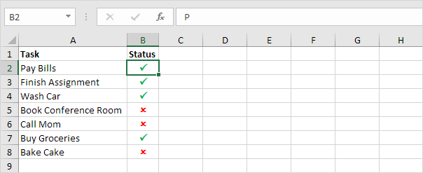
5. Now you can create a nice to-do list that uses check marks. Use CTRL + c and CTRL + v to copy/paste a check mark or red X.

Instead of executing step 1 and 2, you can also use the Insert tab to insert a check mark symbol. Here you can find other symbols as well.

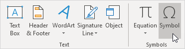
6. On the Insert tab, in the Symbols group, click Symbol.

7. Select Wingdings 2 from the drop-down list, select a check mark and click Insert.

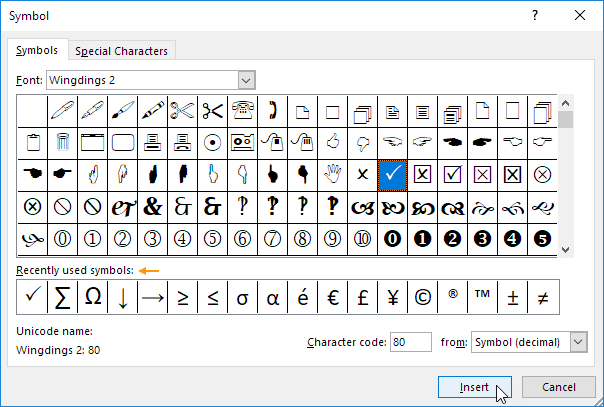
Note: you can also insert a check mark symbol with a box around it (see picture above). After inserting one check mark, you can use the Recently used symbols to quickly insert another check mark.