
Split your worksheet to view multiple distant parts of your worksheet at once. To split your worksheet (window) into an upper and lower part (pane), execute the following steps.
There is a very handy method to split worksheet into panes which just needs to drag the split pane to the location you want to split.
Split worksheet into panes horizontally
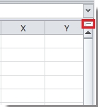
1. Put the cursor at the split bar which is located above the scroll arrow at the top of the vertical scroll bar. See screenshot:
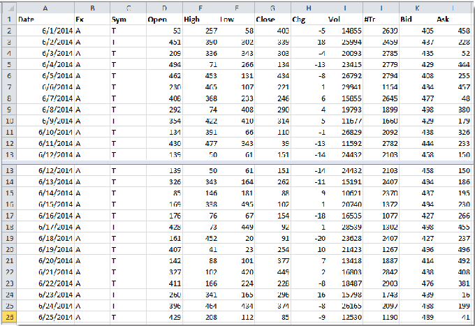
2. Then when the cursor pointer changes to a double-headed arrow with a split in its middle, drag it to the location you want to split the worksheet, and then release the cursor. See screenshot:
Split worksheet into panes vertically
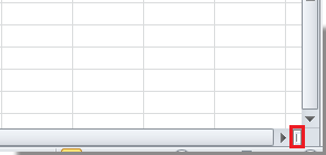
1. Put the cursor at the split bar which is located next to the scroll arrow at the right of the horizontal scroll bar. See screenshot:
2. Then when the cursor pointer changes to a double-headed arrow with a split in its middle, drag it to the location you want to split the worksheet, and then release the cursor. See screenshot:
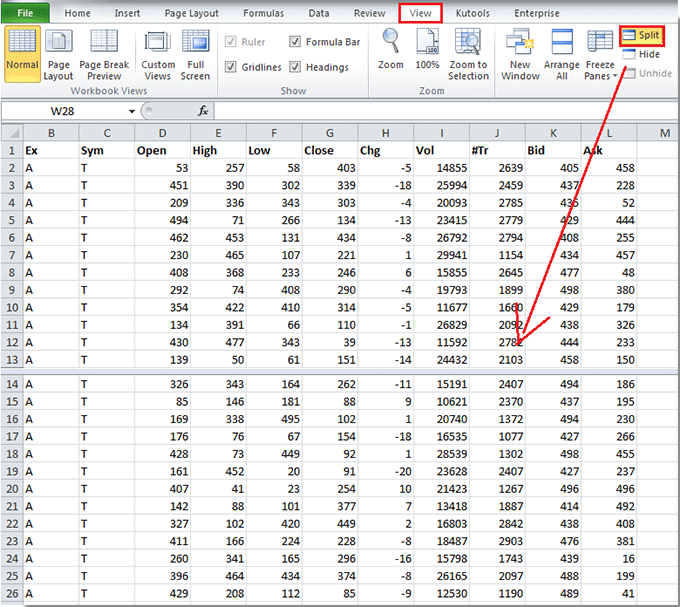
Split Worksheet Into Panes With Split Button
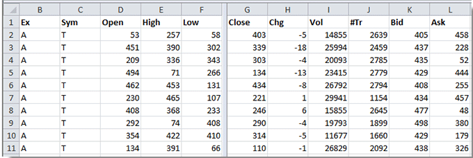
1. First, select a cell in column A.
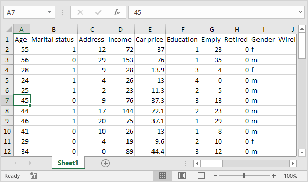
2. On the View tab, in the Window group, click Split.

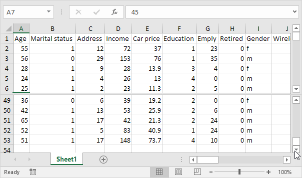
3. Notice the two vertical scroll bars. For example, use the lower vertical scroll bar to move to row 49. As you can see, the first 6 rows remain visible.
4. To change the window layout, use the horizontal split bar that divides the panes.
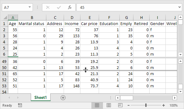
5. To remove the split, simply double click the split bar.
Note: in a similar way, you can split your window into a left and right pane by selecting a cell in row 1 before you click View, Split. You can even split your window into four panes by selecting a cell that is not column A or row 1. Any changes you make to one pane are immediately reflected in the other ones.