Cell Styles

All cell content uses the same formatting by default, which can make it difficult to read a workbook with a lot of information. Basic formatting can customize the look and feel of your workbook, allowing you to draw attention to specific sections and making your content easier to view and understand.

Formatting your Excel spreadsheets gives them a more polished look, and can also make it easier to read and interpret the data, and thus better suited for meetings and presentations. Excel has a collection of pre-set formatting styles to add color to your worksheet that can take it to the next level.

Quickly format a cell by choosing a cell style. You can also create your own cell style. Quickly format a range of cells by choosing a table style.

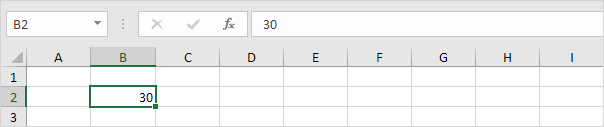
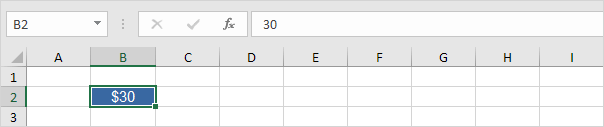
1. For example, select cell B2 below.

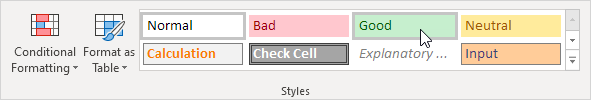
2. On the Home tab, in the Styles group, choose a cell style.

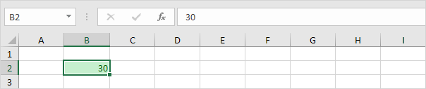
Result.

To create your own cell style, execute the following steps.

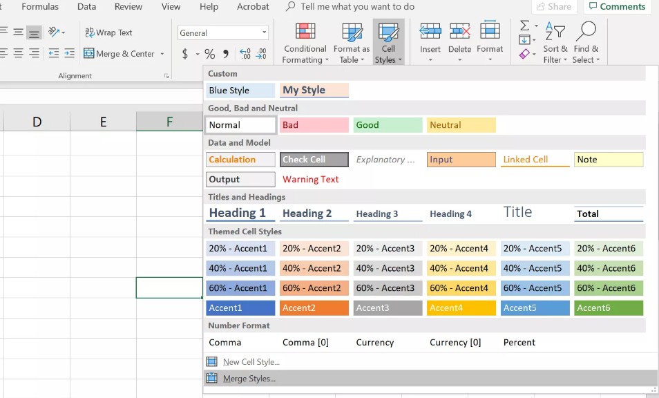
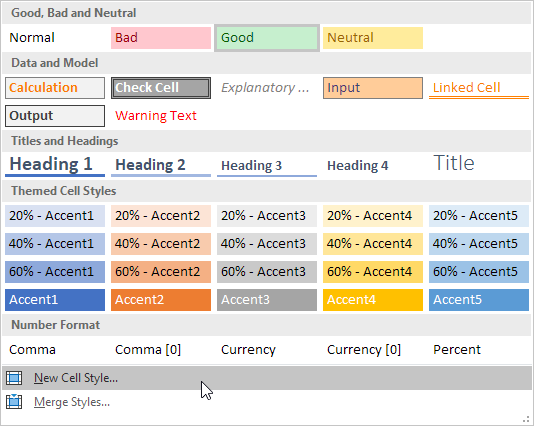
3. On the Home tab, in the Styles group, click the bottom right down arrow.

Here you can find many more cell styles.

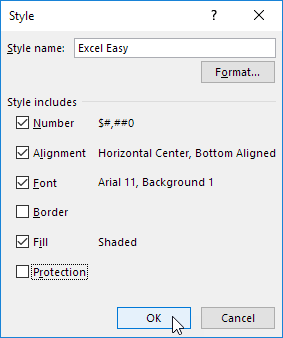
4. Click New Cell Style.

5. Enter a name and click the Format button to define the Number Format, Alignment, Font, Border, Fill and Protection of your cell style. Simply uncheck a check box if you don't want to control this type of formatting.

6. Click OK.

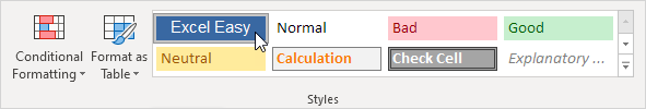
7. On the Home tab, in the Styles group, apply your own cell style.

Result.

Note: right click a cell style to modify or delete it. Modifying a cell style affects all cells in a workbook that use that cell style. This can save a lot of time. A cell style is stored in the workbook where you create it. Open a new workbook and click on Merge Styles (under New Cell Style) to import a cell style (leave the old workbook with the cell style open).