To quickly enter a GETPIVOTDATA function in Excel, type an equal sign (=) and click a cell in a pivot table. The GETPIVOTDATA function can be quite useful.
1. First, select cell B14 below and type =D7 (without clicking cell D7 in the pivot table) to reference the amount of beans exported to France.

2. Use the filter to only show the amounts of vegetables exported to each country.

Note: cell B14 now references the amount of carrots exported to France, not the amount of beans. GETPIVOTDATA to the rescue!
3. Remove the filter. Select cell B14 again, type an equal sign (=) and click cell D7 in the pivot table.

Note: Excel automatically inserts the GETPIVOTDATA function shown above.
4. Again, use the filter to only show the amounts of vegetables exported to each country.

Note: the GETPIVOTDATA function correctly returns the amount of beans exported to France.
5. The GETPIVOTDATA function can only return data that is visible. For example, use the filter to only show the amounts of fruit exported to each country.

Note: the GETPIVOTDATA function returns a #REF! error because the value 680 (beans to France) is not visible.
6. The dynamic GETPIVOTDATA function below returns the amount of mango exported to Canada.

Note: this GETPIVOTDATA function has 6 arguments (data field, a reference to any cell inside the pivot table and 2 field/item pairs). Create a drop-down list in cell B14 and cell B15 to quickly select the first and second item (see downloadable Excel file).
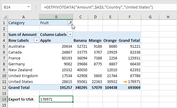
7. The GETPIVOTDATA function below has 4 arguments (data field, a reference to any cell inside the pivot table and 1 field/item pair) and returns the total amount exported to the USA.

8. If the total amount exported to the USA changes (for example, by using a filter), the value returned by the GETPIVOTDATA function also changes.
If you don't want Excel to automatically insert a GETPIVOTDATA function, you can turn off this feature.
9. Click any cell inside the pivot table.
10. On the Analyze tab, in the PivotTable group, click the drop-down arrow next to Options and uncheck Generate GetPivotData.
