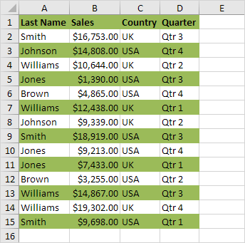
This example shows you how to use conditional formatting to shade alternate rows. Shading every other row in a range makes it easier to read your data.
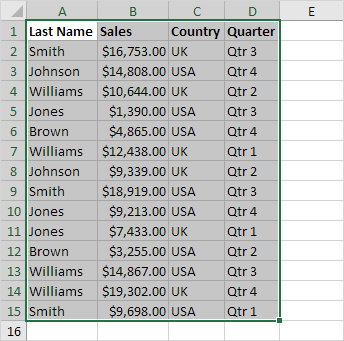
1. Select a range.
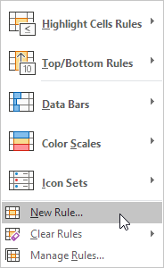
2. On the Home tab, in the Styles group, click Conditional Formatting.

3. Click New Rule.
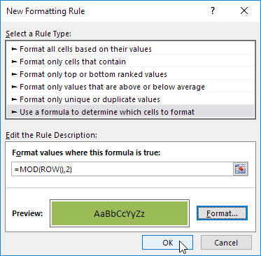
4. Select ‘Use a formula to determine which cells to format’.
5. Enter the formula =MOD(ROW(),2)
6. Select a formatting style and click OK.
Result.

Explanation: the MOD function gives the remainder of a division. The ROW() function returns the row number. For example, for the seventh row, MOD(7,2) equals 1. 7 is divided by 2 (3 times) to give a remainder of 1. For the eight row, MOD(8,2) equals 0. 8 is divided by 2 (exactly 4 times) to give a remainder of 0. As a result, all odd rows return 1 (TRUE) and will be shaded.
