If you want to look up a value in a table using one criteria, it’s simple. You can use a plain VLOOKUP formula. But if you want to use more than one criteria, what can you do? There are lots of ways using several Excel functions such as VLOOKUP, LOOKUP, MATCH, INDEX, etc. In this blog post, I’ll show you a few of those ways.
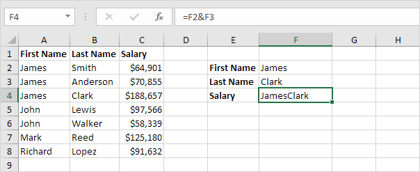
This example teaches you how to perform a two-column lookup in Excel. See the example below. We want to look up the salary of James Clark, not James Smith, not James Anderson.
- To join strings, use the & operator.

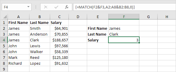
- The MATCH function returns the position of a value in a given range. Insert the MATCH function shown below.
- Finish by pressing CTRL + SHIFT + ENTER.

Note: The formula bar indicates that this is an array formula by enclosing it in curly braces {}. Do not type these yourself. They will disappear when you edit the formula.
Explanation: The range (array constant) A2:A8&B2:B8 is stored in Excel's memory, not in a range. The array constant looks as follows:
{“JamesSmith”;“JamesAnderson”;“JamesClark”;“JohnLewis”;“JohnWalker”;“MarkReed”;“RichardLopez”}
This array constant is used as an argument for the MATCH function, giving a result of 3 (JamesClark found at position 3).
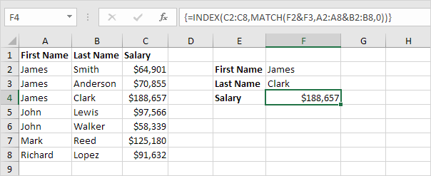
- Use this result and the INDEX function to return the 3rd value in the range C2:C8.

