Freeze Panes in Excel

When you work with a large table, it’s easy to lose headings when you scroll.
Freeze Panes lets you keep important rows or columns always visible while scrolling.

---

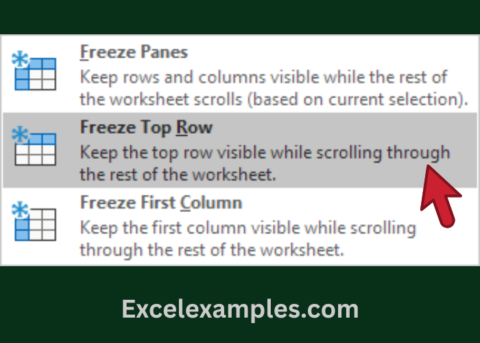
Freeze the Top Row (Most Common)

Use this when your column titles are in Row 1.

1. Click the View tab.
2. In the Window group, click Freeze Panes.
   
   
   
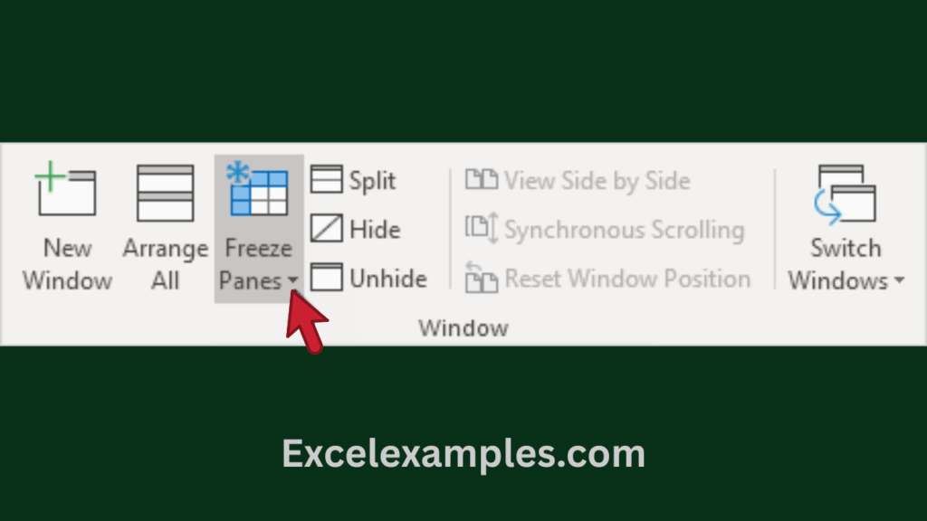
3. Click Freeze Top Row.
   
   
   
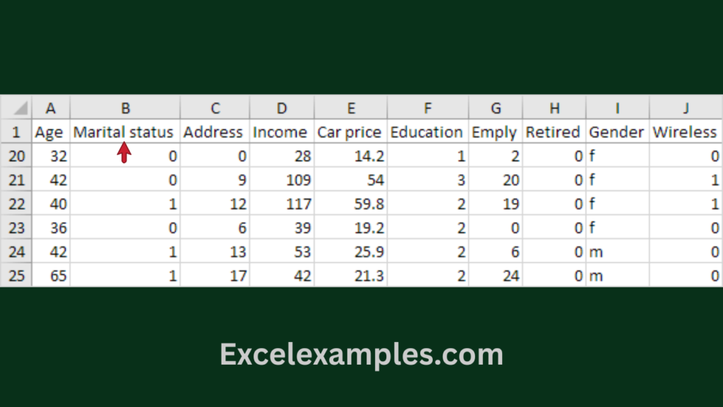
4. Scroll down.

---

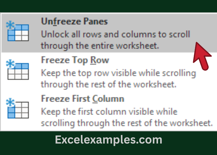
Unfreeze Rows or Columns

Use this to remove all freezes.

1. Click the View tab.
2. Click Freeze Panes.
   
   
   
3. Click Unfreeze Panes.

---

Freeze the First Column

Use this when important labels are in Column A.

1. Click the View tab.
2. Click Freeze Panes.
   
   
   
3. Click Freeze First Column.
   
   
   
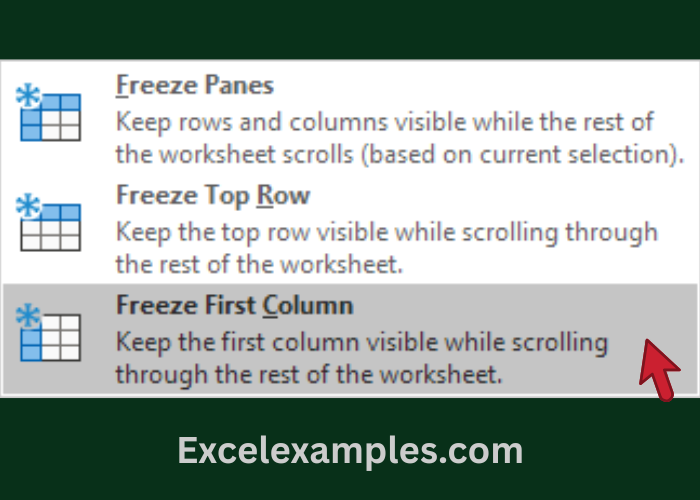
4. Scroll to the right.

---

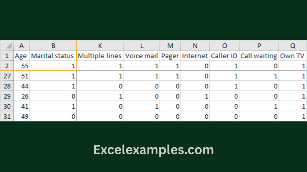
Freeze Multiple Rows (Example: Freeze Rows 1–3)

Rule to remember (very important):
👉 Excel freezes everything ABOVE the selected row

1. Click row 4.
2. Click the View tab.
3. Click Freeze Panes.
   
   
   
4. Click Freeze Panes again.
   
   
   
5. Scroll down.

---

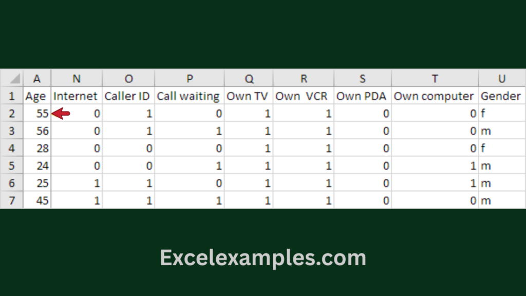
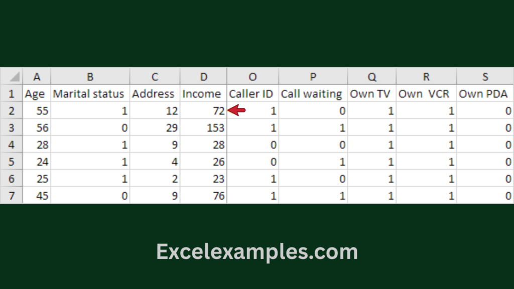
Freeze Multiple Columns (Example: Freeze Columns A–D)

Rule to remember:
👉 Excel freezes everything to the LEFT of the selected column

1. Click column E.
2. Click the View tab.
3. Click Freeze Panes.
   
   
   
4. Click Freeze Panes. Click Freeze Panes again.
   
   
   
5. Scroll right.

---

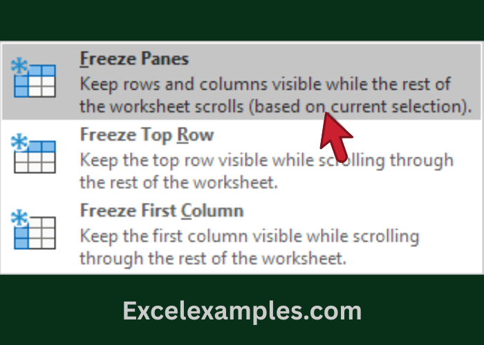
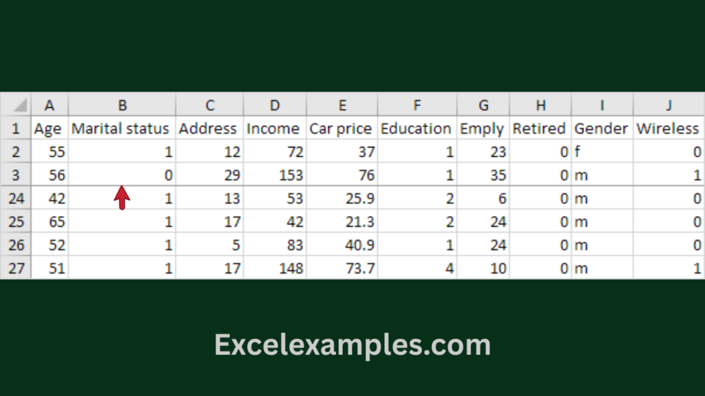
Freeze Rows AND Columns at the Same Time (Freeze Cells)

Use this to lock both headings and labels.

Rule to remember (golden rule 🧠):
👉 Excel freezes everything ABOVE and to the LEFT of the selected cell

Example: Freeze rows 1–2 and columns A–B

1. Click cell C3.
2. Click the View tab.
3. Click Freeze Panes.
   
   
   
4. Click Freeze Panes.
   
   
   
5. Scroll down and right.

---

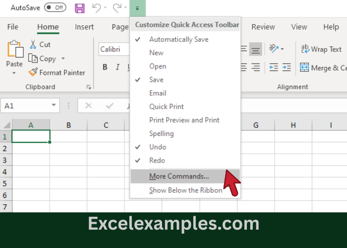
Magic Freeze Button (One-Click Freeze)

You can add Freeze Panes as a quick button.

1. Click the small down arrow on the top-left (Quick Access Toolbar).
2. Click More Commands.
   
   
   
3. Under Choose commands from, select Commands Not in the Ribbon.
4. Select Freeze Panes → click Add.
   
   
   
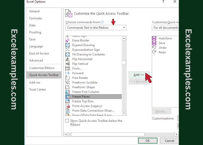
5. Click OK