Dynamic Calendar in Excel

Want to create a calendar that automatically updates when you switch years (from 2025 to 2026, for example)? This guide breaks down the core logic and formulas you need to make it happen.

(Note: This tutorial focuses on the mathematical “engine” behind the calendar. We assume you already know how to style your spreadsheet with background colors, borders, and custom fonts).

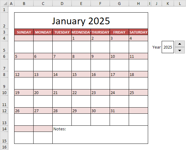
Step 1: Tell Excel When the Month Starts

The biggest hurdle is figuring out exactly what day of the week January 1st falls on. To keep our formulas clean, we will set up two Named Ranges.

Range Name	Cell / Formula	Purpose
CalendarYear	K5 (or any blank cell)	The input cell where you type the target year (e.g., 2025).
JanOffset	=DATE(CalendarYear,1,1) - WEEKDAY(DATE(CalendarYear,1,1))	Calculates the starting anchor date for the calendar grid.

How the JanOffset logic works:

Excel tracks dates as continuous serial numbers starting from January 1, 1900.

• The DATE function calculates the exact serial number for January 1st of your chosen year. For Jan 1, 2025, this number is 45658.
• The WEEKDAY function translates that date into a numerical day of the week (1 is Sunday, 7 is Saturday). Since Jan 1, 2025, is a Wednesday, it returns 4.
• By subtracting the weekday value from the date value (45658 - 4 = 45654), we shift back in time to find the exact date of the Saturday from the previous week. This number, 45654, serves as the anchor point (JanOffset) for the entire calendar.

Step 2: Populate the Calendar Grid

Let’s assume your January layout has Sunday as the first column, starting in cell B4.

1. Formula for the First Sunday (Cell B4):

=IF(AND(YEAR(JanOffset+1)=CalendarYear, MONTH(JanOffset+1)=1), JanOffset+1, "")

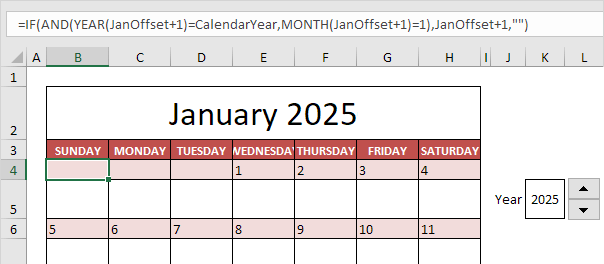
How it works: We add 1 day to our anchor point (JanOffset + 1). The IF function then evaluates whether this specific date actually belongs to January of your selected year. Since this date is likely in late December of the previous year, the formula returns a completely blank cell ("").

2. Formula for the First Wednesday (Cell E4):

Moving across the row to the Wednesday column, the formula becomes:

=IF(AND(YEAR(JanOffset+4)=CalendarYear, MONTH(JanOffset+4)=1), JanOffset+4, "")

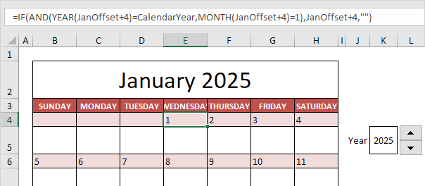
How it works: By adding 4 days to the anchor (JanOffset + 4), we land exactly on January 1, 2025! Because this date satisfies the condition of being in January of our target year, Excel successfully displays the date.

You simply repeat this sequential progression (adding 2, 3, 5, etc., to the offset) to populate the remaining days of the month.

Step 3: Format Cells to Display the Day Only

At this point, your grid cells are showing full dates like “1/1/2025”. To make it look like a traditional calendar, we need to hide the month and year data.

1. Highlight your entire calendar grid.
2. Press Ctrl + 1 to launch the Format Cells window.
3. Navigate to the Number tab and choose Custom from the list.
4. In the “Type” input box, delete the existing text and type a single d.
5. Click OK.

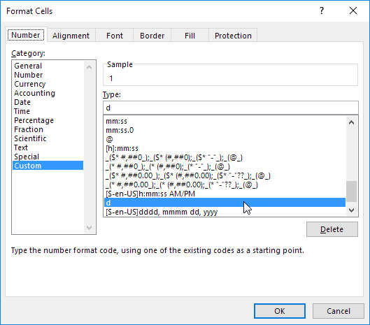
Immediately, a cell containing “1/1/2025” will visually shrink to show just the number 1.

Pro Tip: Apply this exact same methodology to generate the remaining 11 months. To make it even more interactive, insert a Spin Button from the Developer tab and link it to your CalendarYear cell. This allows you to effortlessly toggle through past and future years with a single click!