In Excel, Currency and Accounting formats are used to display money values.
They look similar, but they behave slightly differently.

---

1. Apply Currency Format

Step 1: Select the cells

Select the range of cells that contains numbers.

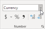
Step 2: Apply the format

Go to: Home → Number group → Currency

Shortcut: Ctrl + Shift + 4

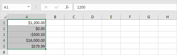
Result

The Currency format displays the currency symbol right next to the number.

---

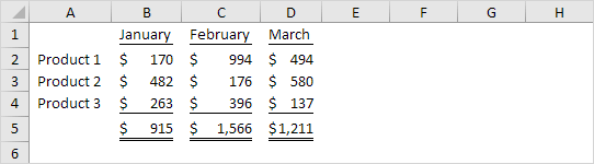
2. Apply Accounting Format

Step 1: Select the cells

Select the same range.

Step 2: Apply Accounting format

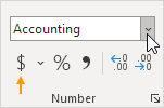
Go to: Home → Number group → Accounting

Or simply click the $ button.

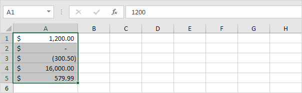
Result

The Accounting format:

• Aligns currency symbols in a column
• Aligns decimal points
• Shows zero values as a dash (—)
• Displays negative numbers in parentheses

---

Main Difference

Currency	Accounting
Symbol is next to the number	Symbol is aligned in a column
Zero appears as 0.00	Zero appears as —
More flexible negative formats	Usually shows negatives in parentheses

---

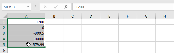
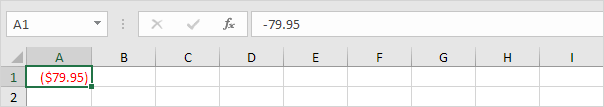
3. Format Negative Numbers

You can customize how negative numbers appear.

Steps

1. Select a cell with a negative number.
2. Right-click the cell.
3. Click Format Cells (or press Ctrl + 1).
4. Choose Currency.
5. Under Negative Numbers, select a style.

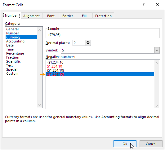
Result:

---

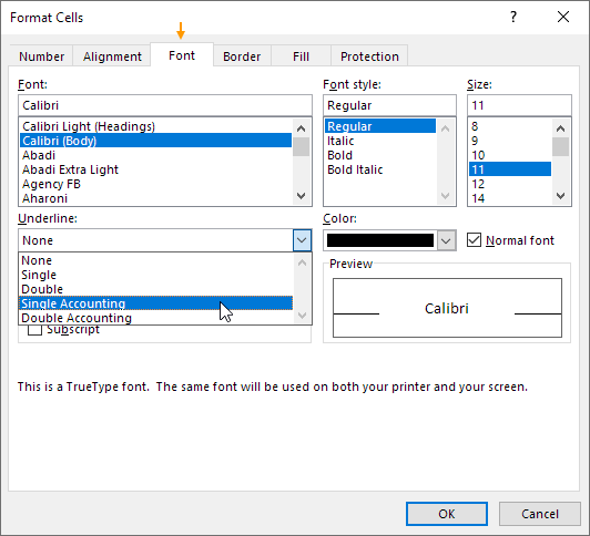
4. Use Accounting Underlines

Excel also has special underlines used in financial reports.

1. Press Ctrl + 1 to open Format Cells.
2. Go to the Font tab.
3. Choose:

• Single Accounting underline
• Double Accounting underline

These are often used in financial statements and reports.